Meteorological Derived Parameters¶

POWER provides value-added products from core meteorological parameters for POWER community use. Equations/methods for producing these parameters are presented below, along with validation of these parameters as possible.

Relative Humidity¶

The relative humidity (RH) values in the POWER Archive are calculated from pressure (P_a in kPa), dry-bulb temperature (T_a in °C), and specific humidity (q in kg/kg), parameters that are available from the re-gridded MERRA-2 and represents estimates at two meters above the local surface averaged over the original source spatial resolution. The following is a summary of the expressions used to calculate RH. The units are indicated in square brackets. MERRA-2 (see meteorological section in these documents for more information on MERRA-2) provides two-meter air temperature, specific humidity, and surface pressure needed to derive humidity quantities. Relative humidity is conventionally defined as the ratio of the actual to the saturation water vapor pressure at the ambient temperature.

Equation¶

Following Murphy and Koop, 2005 Relative humidity is calculated by:

$\begin{align} RH = (e_a/e_{sat}) \times 100 \text{[%]} \tag {Equation 1} \end{align}$

$\begin{align} Where: \\ e_a: & \text{ the water vapor pressure }\\ e_{sat}: & \text{ the saturation water vapor pressure at the ambient temperature $T_a$.}\\ \end{align}$

$\begin{align} \text{The 100 has been added to cast RH in terms of percent.} \end{align}$

$\begin{align} e_a = (10 \times P_a \times w)/(\varepsilon + w) \text{ } [hPa] \tag {Equation 2} \end{align}$

$\begin{align} Where: \\ w: & \text{ mixing ratio define as the ratio of mass of water to dry air }\\ \end{align}$

$\begin{align} ϵ = \frac{R'}{R_v} = \frac{287.05}{461.5} ≃ 0.622 \tag {Equation 3} \end{align}$

$\begin{align} Where: \\ R': & \text{ Dry vapor gas constant }\\ R_v: & \text{ Water vapor gas constant } \end{align}$

$\begin{align} w = q / (1-q) \text{ } [kg/kg] \tag {Equation 4} \end{align}$

Combining Equation 2 and Equation 4 leads to the following expression for $e$ in terms of $q$ :

$\begin{align} e_a = q \times 10 \times P_a / [\varepsilon + q \times (1- \varepsilon)] \text{ } [hPa] \tag {Equation 5} \end{align}$

An eighth-order polynomial fit (Flatau et al., 1992) to measurements of vapor pressure over ice and over water provides an expression to calculate the saturated water vapor pressure. The eighth-order fit for $e_{wsat}$ is given by:

$\begin{align} e_{wsat} & = A_{1w} + A_{2w}×(T_a) + …+ A_{(n-1)w}×(T_a)^n \tag {Equation 6} \\ e_{isat} & = A_{li} + A_{2i}×(T_a) + …+ A_{(n-1)i}×(T_a)^n \tag {Equation 7} \end{align}$

$\begin{align} Where: \\ e_{wsat}: & \text{ Saturated vapor pressure over water in [hPa = mb] }\\ e_{isat}: & \text{ Saturated vapor pressure over ice [hPa = mb] }\\ T_a: & \text{ Ambient dry bulb temperature in °C } \end{align}$

Coefficients¶

Coefficients for $e_{sat}$ over water and over ice and the temperature range over which the coefficient are applicable

Over Water (Valid: -85 °C to 70 °C)	Over Ice (Valid: -90 °C to 0 °C)
A1w = 6.11583699	A1i = 6.09868993
A2w = 0.444606896	A2i = 0.499320233
A3w = 0.143177157E-1	A3i = 0.184672631E-1
A4w = 0.264224321E-3	A4i = 0.402737184E-3
A5w = 0.299291081E-5	A5i = 0.565392987E-5
A6w = 0.203154182E-7	A6i = 0.521693933E-7
A7w = 0.702620698E-10	A7i = 0.307839583E-9
A8w = 0.379534310E-13	A8i = 0.105758160E-11
A9w = -0.321582393E-15	A9i = 0.161444444E-14

Note

Only the relative humidity over water is calculated and provided in the POWER Archive consistent with the values reported by the National Weather Service.

Validation¶

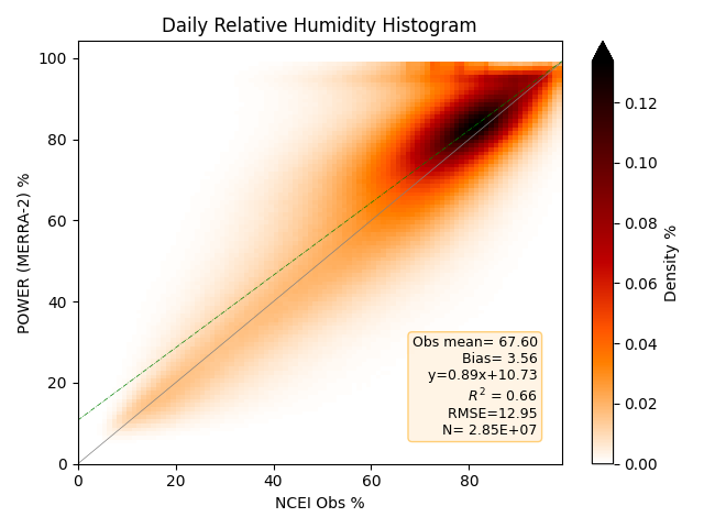
Daily Relative Humidity

Density plot of the 2-D histograms comparing MERRA-2 daily relative humidity with station-derived values from observations from the selected NCEI ISD files for the years 2001–2023. Darker reds indicate a higher number of matched pairs within the 2-D histogram. Both POWER RH and NCEI RH are derived from respective dry bulb and dew point values using the relationships discussed above.

Daily Relative Humidity

Wet Bulb Temperature¶

The wet bulb temperature (T2MWET) calculations use a numerical root-finding approach to solve the standard psychrometric equation. Because the psychrometric equation cannot be solved algebraically for the wet bulb temperature, this method uses a Bisection Algorithm to iteratively find the exact thermodynamic wet bulb temperature that balances the vapor pressure equations (using Murphy and Koop, 2005, from above). Unlike empirical approximations (which are only accurate within limited temperature and humidity ranges), this iterative approach provides highly accurate results across a wide range of atmospheric conditions by relying on foundational thermodynamic principles.

Wet Bulb Algorithm

The methodology employs a bisection loop that continuously narrows down the possible range of the wet bulb temperature until it converges on the true value.

Inputs: Dry Bulb Temperature (T2M) Dew Point Temperature (T2MDEW): Used to establish the lower bound and calculate actual vapor pressure Atmospheric Surface Pressure (PS)

Step 1: Establish Physical Bounds By definition, the wet bulb temperature must be less than or equal to the dry bulb temperature, and greater than or equal to the dew point temperature. Maximum Bound ( $T_{max}$ ): Set to the Dry Bulb Temperature. Minimum Bound ( $T_{min}$ ): Set to the Dew Point Temperature.

Step 2: Calculate Midpoint (The Guess) The algorithm guesses the wet bulb temperature ( $T_{guess}$ ) by finding the exact midpoint between the current minimum and maximum bounds: $T_{guess} = \frac{T_{max} + T_{min}}{2}$

Step 3: Evaluate the Psychrometric Equation Using the estimated wet bulb temperature ( $T_{guess}$ ), the dry-bulb temperature ( $T_{dry}$ ), the standard psychrometric constant [0.00066 K{-1}] and the atmospheric pressure (P), the algorithm calculates the expected psychrometric pressure difference ( $P_{eq}$ ): $P_{eq} = 0.00066 \times (1.0 + 0.00155 \times T_{guess}) \times P \times (T_{dry} - T_{guess})$ It then compares the saturated vapor pressure at the estimated wet bulb temperature against the actual vapor pressure of the air.

Step 4: Check for Convergence The algorithm calculates the difference (residual error) between the calculated pressures. If the absolute difference is less than the strict tolerance threshold (e.g., < 0.01), the model has successfully converged. The current guess ( $T_{guess}$ ) is recorded as the final Wet Bulb Temperature, and the loop terminates.

Step 5: Adjust Bounds (Bisection) If the model has not converged, it evaluates the sign of the difference: If the difference is less than zero, the guessed temperature was too high. The maximum bound ( $T_{max}$ ) is updated to the current guess. If the difference is greater than zero, the guessed temperature was too low. The minimum bound ( $T_{min}$ ) is updated to the current guess.

The loop repeats from Step 2, halving the search space with every iteration, guaranteeing rapid and stable convergence.

Moist Air Enthalpy¶

Specific enthalpy (ENTHALPY) calculations determine the total heat content of a moist air parcel (expressed in kilojoules per kilogram of dry air, $kJ/kg$ ). The algorithm computes this by summing the sensible heat of the dry air and the total heat (sensible plus latent) of the water vapor contained within that air.

Equation¶

$\begin{align} W = 0.621945 \times \left( \frac{e}{P_{s} - e} \right)\\ h = (c_{pa} \times T) + W \times (c_{pw} \times T + L_{w}) \end{align}$

$\begin{align} Where: \\ h: & \text{ enthalpy }\\ W: & \text{ mixing ratio }\\ e: & \text{ vapor pressure of air }\\ P_{s}: & \text{ Surface Pressure}\\ c_{pa}: & \text{ specific heat capacity of dry air = 1.006 kJ/(kg °C) }\\ c_{pw}: & \text{ specific heat capacity of water vapor at constant pressure = 1.86 kJ/(kg °C) }\\ L_{w}: & \text{ latent heat of vaporization at water at 0°C = 2501 kJ/(kg) }\\ T: & \text{ air temperature }\\ \end{align}$

Heating/Cooling Degree Days¶

An important application of historical temperature data is in the calculation of Heating Degree Days (HDD) and Cooling Degree Days (CDD). Degree-day indices are the integrated departure of daily mean temperature from a base temperature and are widely used to estimate building heating and cooling energy demand. The following expressions are used herein for calculating HDD and CDD (Chapter 14 of ASHRAE, 2013):

Equation¶

\begin{align} T_{i} = (T_{max} + T_{min})/2 \tag {Equation 1} \end{align}

$\begin{align} Where: \\ T_{i}: & \text{ The daily mean temperature from the 24 hourly components. }\\ T_{max}: & \text{ The daily maximum temperature from the 24 hourly components. }\\ T_{min}: & \text{ The daily minimum temperature from the 24 hourly components. } \end{align}$

\begin{align} HDD = \sum(T_{base} - T_i )^+ \tag {Equation 2} \end{align}

\begin{align} CDD = \sum( T_i - T_{base})^+ \tag {Equation 3} \end{align}

The "+" superscript in the above equations indicates that only the positive values of the operation in the parenthesis are taken into account in the sum. The sum is taken from i = 1 to N, where N is number of days in the given time period. POWER provides HDD and CDD values for $T_{base}$ = 0 °C, 10 °C, and 18.3 °C.

Validation¶

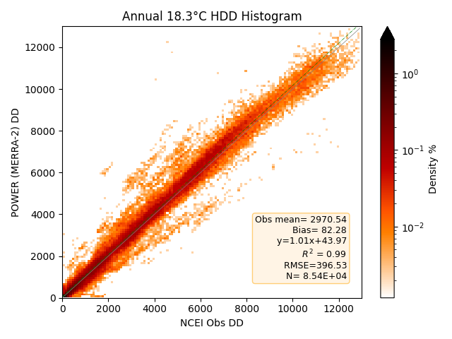
Validations of HDD

HDDSites with Minimal Elevation Difference

Density plot of the 2-D histograms comparing the calculated heating degree days from MERRA-2 with those calculated from station observations from the NCEI GSOD files for 1981–2023. Darker reds indicate a higher number of matched pairs within the 2-D histogram. Note that the color scale is logarithmic to show more bins, as the densest bins are near the origin.

Heating Degree Days 18.3

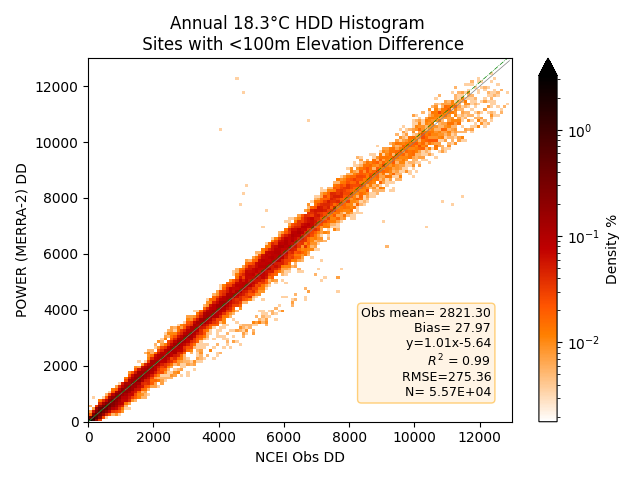
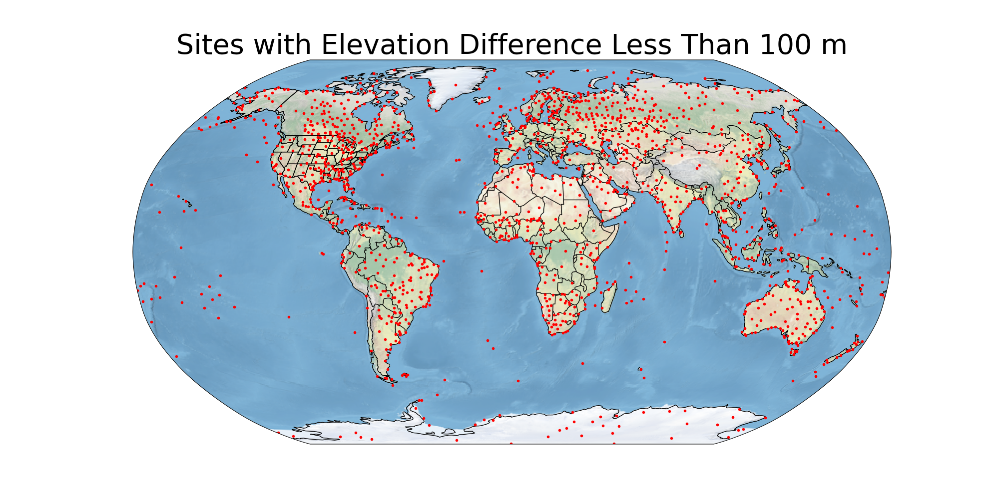
Like the Previous Validation Study (see info box below), this is the histogram for the surface sites with MERRA-2 elevation within 100 m of the station elevation.

Heating Degree Days 18.3, within 100 m

Validations of CDD

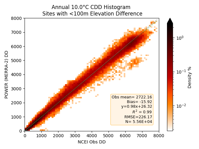
CDDSites with Minimal Elevation Difference

Density plot of the 2-D histograms comparing the calculated cooling degree days from MERRA-2 with those calculated from station observations from the NCEI GSOD files for 1981–2023. Darker reds indicate a higher number of matched pairs within the 2-D histogram. Note that the color scale is logarithmic to show more bins, as the densest bins are near the origin.

Cooling Degree Days 10.0

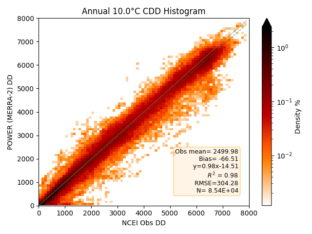
Like the Previous Validation Study (see info box below), this is the histogram for the surface sites with MERRA-2 elevation within 100 m of the station elevation.

Cooling Degree Days 10.0, within 100 m

Map of Sites with Elevation Difference Less Than 100 m

Sites with elevation difference < 100 m

Previous Validation Study

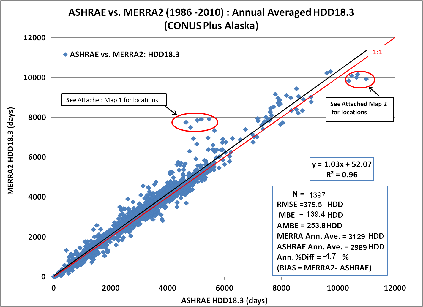
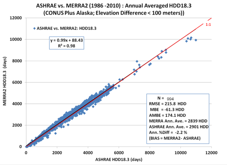
Alaska Anomalies (HDD)Similar Elevation Sites (HDD)CDD

Heating Degree Days 18.3

The scatter plot of the HDD $T_{base}$ = 18.3 °C, shown above, calculated via Equation 2 using the MERRA-2 temperatures versus the corresponding HDD values taken from the American Society of Heating, Refrigerating and Air-Conditioning Engineers (ASHRAE) Weather Data Viewer version 5.0 (WDV 5.0). The WDV values are based upon surface observations over the time period 1986–2010; the MERRA-2 values correspond to the temperature for the MERRA-2 0.5° grid cell around the given surface site. The scatter plot above encompasses 1,397 surface grid pairs in the continental US (CONUS) and Alaska.

TODO[SCIENCE|High]: Report the uncertainty for the 1,397-pair HDD/CDD comparison (bias, RMSE, correlation, and confidence interval) alongside the stated sample size.

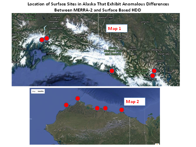
While the overall agreement is good, note the cluster of data point circled in the middle and the upper right portion of the scatter plot. These data are associated with the surface sites shown on maps 1 and 2 below, and are highlighted to call attention to two aspects of the MERRA-2 data that can be problematic depending on the application. Recall that the MERRA-2 values represent the average over their original source spatial resolution. Accordingly, in mountainous regions (e.g., map 1) the average elevation of the MERRA-2 cell can be significantly different from the elevation of the local surface site. Similarly, in regions where the surface temperatures may have strong horizontal gradients, such as near coast lines (e.g., map 2) the average temperature of the MERRA-2 cell can be different than the local station.

Location of surface sites for HDD and CDD

The scatter plot and associated statistics for the same stations used when the elevation difference between the surface site and the MERRA-2 grid is less than 100 m.

Scatter Plot Less than 100 m

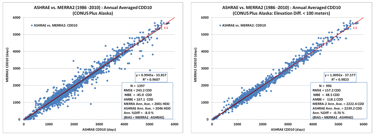
The left and right scatter plots below show the corresponding scatter plots for CDD with $T_{base}$ = 10 °C.

Scatter Plot for Site Comparison

Growing Degree Days¶

Another application of temperature data is in the usage of Growing Degree Days (GDD). GDD, like HDD and CDD, are based upon the deviation of the daily averaged temperature, typically evaluated as $(T_{max}$ + $T_{min})/2$ , relative to a reference temperature, $T_{base}$ . GDD are measures of the heat accumulation of a location which allow prediction of different growth stages of crops and emergence of insects. The following equations are used by POWER to calculate the daily GDD:

Equation¶

\begin{align} T_{min} = max(T_{min},T_{base}) \tag {Minimum Daily Temperature adjustment} \end{align}

$\begin{align} T_{i} = (T_{max} + T_{min})/2 \tag {Equation 1} \end{align}$

\begin{align} GDD = max(T_{i}-T_{base},0) \tag {Equation 2} \end{align}

$\begin{align} Where: \\ T_{i}: & \text{ The base temperature, dependent on plant/insect type. }\\ T_{base}: & \text{ The daily mean temperature from the 24 hourly components. }\\ T_{max}: & \text{ The daily maximum temperature from the 24 hourly components. }\\ T_{min}: & \text{ The daily minimum temperature from the 24 hourly components. } \end{align}$

Available Growing Degree Day Base Temperatures

Crop	Temp (°C)	Temp (°F)	Parameter Name
Cotton	15.6	60.0	GDD15_6
Peanut	13.3	56.0	GDD13_3
Corn, sweet corn, sorghum, rice, soybeans, beans	10.0	50.0	GDD10
Potato, sunflower	7.2	45.0	GDD7_2
Wheat, barley, rye, oats, canola, lettuce	4.4	40.0	GDD4_4